The Problem With Words and Computers
Computers are deeply uncomfortable with language. At the hardware level, everything is numbers. Text, as humans write it, is just a sequence of arbitrary tokens with no intrinsic numeric relationship. The word “dog” isn’t closer to “puppy” than it is to “carburetor” unless you explicitly encode that relationship somewhere.
For decades, the standard approach was to encode text as sparse vectors. A vocabulary of 100,000 words becomes a vector with 100,000 dimensions. Each word is a point in that space with a 1 in exactly one position and zeros everywhere else. This is called one-hot encoding, and it has a severe limitation: every word is exactly as far from every other word. “King” and “queen” are just as distant as “king” and “asphalt.” The representation carries no semantic information at all.
Embeddings are the solution to this. The core idea is to represent tokens (words, sentences, images, audio, whatever) as dense vectors in a much lower-dimensional space, where the geometry of that space reflects meaning. Things that are semantically similar end up close together. Things that are semantically different end up far apart. And crucially, the directions in that space can encode relationships.
This isn’t a new idea. It’s roughly as old as neural networks themselves. But it’s the idea that almost everything interesting in modern AI is built on top of.
Word2Vec and the Moment It Clicked
The concept became concrete for a lot of people in 2013 when Google researchers published Word2Vec. The paper described a family of techniques for training a shallow neural network on massive amounts of text, where the objective was to predict a word from its surrounding context (or vice versa). The actual outputs of interest weren’t the predictions. They were the learned internal representations: 300-dimensional vectors for each word in the vocabulary.
These vectors had a property that felt almost magical: arithmetic worked on them semantically. The classic example is vector("king") - vector("man") + vector("woman") produces a vector very close to vector("queen"). The geometry of the space had captured an actual relationship. Royalty minus maleness plus femaleness points toward female royalty. This wasn’t programmed in. It emerged from training a network to predict words from context across billions of examples.
It worked because of distributional semantics, the observation (originally from linguist John Firth in the 1950s) that words appearing in similar contexts tend to have similar meanings. The network, trained to predict context, was forced to learn representations that captured those contextual patterns. Similar context patterns produced similar vectors.
Think of it this way. If you read enough text, you notice that “dog” and “puppy” appear in similar sentence structures, surrounded by similar words, in similar topics. A network optimized to predict context will represent them similarly because that’s the efficient solution. The geometry falls out as a byproduct of doing the prediction task well.
How Embeddings Are Actually Trained
The mechanics are worth understanding, because the training objective shapes everything about what the resulting embeddings capture.
In a basic word embedding setup, you define a context window (say, five words on each side), slide it across your training corpus, and generate training examples of the form “given this center word, predict these surrounding words” or “given these surrounding words, predict the center word.” The network learns a weight matrix that maps one-hot vocabulary vectors to dense vectors, and another matrix that maps them back. The dense vectors in the middle layer are the embeddings.
Backpropagation (the algorithm for adjusting weights based on prediction errors) nudges the embeddings of words that appear in similar contexts to be more similar. After enough training, the embedding space organizes itself by meaning.
Modern embedding models are more sophisticated. Sentence transformers, for instance, are built on top of transformer architectures and are trained on pairs of sentences labeled as semantically similar or dissimilar. The model learns to map entire sentences (not just words) to vectors, such that semantically similar sentences cluster together. Models like OpenAI’s text-embedding-ada-002 or the open-source sentence-transformers library produce embeddings this way. You pass in a string, you get back a vector of 768 or 1536 floats, and that vector encodes the meaning of the string in a form the machine can actually compute with.
What You Can Do With a Vector of Meaning
Once you can represent meaning as vectors, a lot of useful operations become simple geometry.
Similarity search is the obvious one. Cosine similarity (the angle between two vectors) gives you a fast, meaningful similarity score between any two pieces of text. This is how semantic search works: you embed a query, embed your documents, and find the documents whose vectors are closest to the query vector. Unlike keyword search, which requires lexical overlap, semantic search finds documents that mean the same thing even when they use different words.
This is also the mechanism behind retrieval-augmented generation (RAG), which is the dominant architecture for grounding large language models in external knowledge. You pre-embed a knowledge base, embed the user’s question at query time, retrieve the most relevant chunks, and stuff them into the model’s context. The quality of the retrieval depends almost entirely on the quality of the embeddings. Weak embeddings mean the wrong chunks get retrieved, and the model answers from irrelevant or missing context.
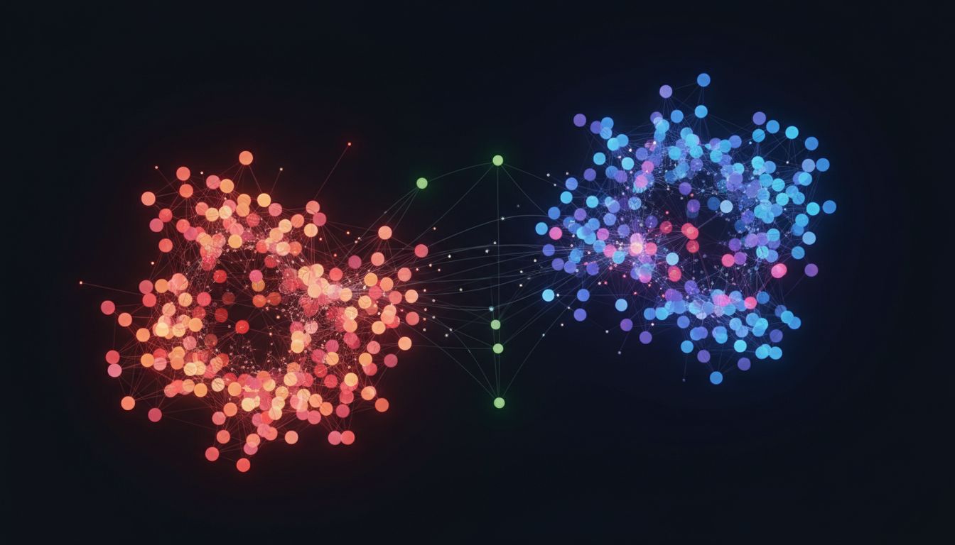
Classification becomes tractable because embedded items that belong to the same category tend to cluster. You can train a simple linear classifier on top of embeddings and get strong results with a fraction of the labeled data you’d need otherwise. The embeddings handle the heavy lifting of representation; the classifier just learns where to draw lines in that space.
Anomalies stand out because embedding distance is a proxy for familiarity. A document or data point with an embedding that’s far from everything in your training distribution is suspicious in a meaningful way.
Recommendation systems use embeddings for both items and users, then recommend items whose vectors are close to the user’s vector. Spotify’s recommendation infrastructure does something close to this, representing users and songs in a shared embedding space. (There’s more detail on that approach in how Spotify learned what songs mean, not just what they are.)
The Role of Vector Databases
Storing and searching through millions of embedding vectors efficiently is a non-trivial problem. Exact nearest-neighbor search in high-dimensional space is expensive. If you have a million vectors at 1536 dimensions each, brute-forcing every query is too slow for interactive use.
Vector databases (Pinecone, Weaviate, Qdrant, pgvector for Postgres users) solve this with approximate nearest neighbor algorithms. Techniques like HNSW (Hierarchical Navigable Small World graphs) build index structures that let you find approximate nearest neighbors in logarithmic rather than linear time, trading a small amount of recall for significant speed improvements.
The word “approximate” is doing real work there. You might miss a small fraction of the truly closest vectors in exchange for a 100x speedup. Whether that tradeoff is acceptable depends entirely on your application. For most recommendation and search use cases, it’s fine. For anything where missing a relevant document has serious consequences, you need to think harder about it.
If you’re evaluating whether to add a vector database to your stack, the decision hinges on whether you’re actually doing semantic similarity search at scale. Many teams reach for specialized vector stores before they’ve proven the need. A focused look at that decision is worth reading before you commit to one.
Embeddings Aren’t Just for Text
The text examples dominate the discourse, but the embedding idea applies wherever you can define a meaningful similarity relationship and collect enough data to learn it.
Images are embedded using convolutional or transformer-based vision models. The penultimate layer of an image classifier, before the final softmax, is an embedding: a dense vector that encodes visual content in a way that’s invariant to small transformations. Image search, visual similarity, and multimodal retrieval all depend on this.
Multimodal embeddings (CLIP being the well-known example from OpenAI, published in 2021) go further: they train a model to place images and their text descriptions close together in a shared embedding space. This is how you can search for images with text queries and get sensible results. The model has learned that a photo of a dog and the text “a dog in a park” should occupy roughly the same region of the space.
Code can be embedded too. Models trained on code-comment pairs learn embeddings where code and its natural language description are nearby. This is how code search tools like GitHub Copilot’s semantic search find relevant snippets from natural language queries.
Audio, molecular structures, user behavior sequences, graph nodes: if you can construct a meaningful similarity criterion and collect training data that reflects it, you can train embeddings. The abstraction is genuinely general.
Limitations Worth Taking Seriously
Embeddings encode the biases in their training data, and they do it silently. Word2Vec trained on 2013 web text reflected the gender biases of that text: professions associated with men were embedded closer to “he” and professions associated with women closer to “she.” The embedding space is a compressed representation of the patterns in the training corpus, including the problematic ones.
Embeddings also struggle with negation and fine-grained logical distinctions. “The patient has no history of heart disease” and “the patient has a history of heart disease” might embed similarly because they share almost all the same words in similar positions. Sentence-level embeddings average over a lot of detail. This matters a lot in high-stakes domains.
Stale embeddings are a real operational problem. If your product catalog changes and you don’t re-embed, your similarity search returns results that don’t reflect the current state of your data. The embedding is a snapshot, not a live view.
Finally, interpreting embeddings is hard. You can measure distances and find neighbors, but understanding why two things are close or far requires probing experiments. This opacity makes debugging embedding-dependent systems genuinely difficult. When retrieval goes wrong, diagnosing whether the problem is the embedding model, the index, the chunking strategy, or the query formulation requires methodical elimination.
What This Means
If you step back, embeddings are a bet on a specific idea: that meaning can be captured as position in space, and that the geometry of that space can be learned from patterns in data. That bet has paid off more than almost anyone expected.
The practical upshot is that a large fraction of what modern AI systems do, from search to recommendations to retrieval-augmented generation to zero-shot classification, reduces to: embed things, then compute distances. Understanding that substrate makes the rest of the AI stack much less mysterious. When something doesn’t work, you can reason about whether the embedding space reflects the similarity relationship you actually care about. When you’re evaluating a new AI product feature, you can ask what the embedding model was trained on and whether that matches your domain.
The idea is deceptively simple. Turn things into vectors such that distance means similarity. Everything else is a consequence.