The Simple Version
A widely-memorized table of computer latency numbers, popularized by Jeff Dean and Peter Norvig around 2012, has become a kind of sacred text in software engineering, but the hardware it describes has changed enough that several of its figures are now off by an order of magnitude or more.
Where the Numbers Come From
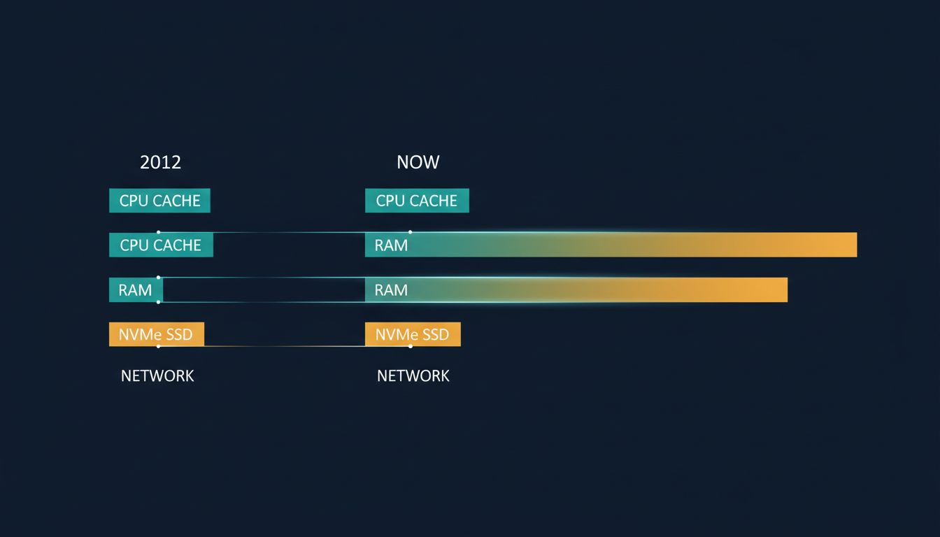
If you’ve been through a systems design interview in the last ten years, you’ve seen the list. L1 cache reference: 0.5 nanoseconds. Main memory reference: 100 nanoseconds. SSD random read: 150 microseconds. A packet round-trip from California to the Netherlands: 150 milliseconds. The numbers feel authoritative because they came from authoritative people: Jeff Dean, who built much of Google’s infrastructure, and Peter Norvig, one of the most respected figures in computer science. They were accurate, or close enough, for the hardware of their era.
That era was roughly 2012. The numbers have been copied, slide-decked, and blog-posted ever since, mostly without revision.
This matters because engineers use these figures to make real decisions: whether to add a caching layer, whether a database query is fast enough, whether a cross-region call is worth the cost. Calibrating those decisions against hardware that no longer exists is a quiet source of architectural drift.
What Has Actually Changed
NVMe storage is the clearest example of the problem. The 2012 table lists SSD random read at around 150 microseconds. A modern NVMe drive, which has been commodity hardware for several years now, delivers random reads closer to 20-100 microseconds, with high-end drives pushing below 20. That’s a 3x to 7x improvement. The old figure isn’t ballpark-wrong; it’s category-wrong. It describes a device class that most new systems no longer use.
Memory bandwidth has shifted too. DDR4, and now DDR5, deliver substantially higher bandwidth than the DDR3 assumed in the original table. Sequential memory access patterns that were once bottlenecked on bandwidth are now more often bottlenecked on cache coherence or software overhead.
Network latency within a single cloud availability zone has dropped considerably. In practice, well-tuned inter-service calls within the same AWS or GCP zone can run in the low hundreds of microseconds, sometimes lower, depending on the networking stack. The original table’s figures for network hops remain roughly correct for wide-area traffic, which is one reason the cross-continental round-trip numbers have aged better than the storage numbers.
CPU cache behavior is where the numbers get genuinely treacherous. Modern processors with large L3 caches change the calculus for data structure design in ways the original table doesn’t capture. A working set that would have been a cache miss in 2012 might now fit comfortably in L3. Engineers who learned to fear cache misses absolutely may be over-engineering for a problem that’s shrunk.
The Numbers That Haven’t Changed Much
Physics is physics. The speed of light across a fiber cable from California to the Netherlands hasn’t changed. Human perception thresholds haven’t changed. The fundamental instruction latency of a branch prediction miss is still in the low nanosecond range. Wide-area network latency is still dominated by distance and routing, not hardware generation.
This creates an asymmetry worth internalizing: the numbers closest to the hardware, where engineering has had the most to work with, have improved the most. The numbers governed by geography and physics have barely moved. If your mental model gets these two categories confused, you’ll over-optimize for storage and under-optimize for network placement.
The Problem with Memorizing Numbers at All
The deeper issue isn’t that engineers have the wrong numbers memorized. It’s that the exercise of memorizing a specific table encourages false precision. Real systems don’t behave like idealized hardware benchmarks. An NVMe read at 30 microseconds in a benchmark can become a 2-millisecond operation in production when you factor in filesystem overhead, kernel scheduler latency, and the specific access pattern of your workload.
The engineers who use latency intuition most effectively don’t recite numbers. They understand orders of magnitude and the relationships between layers. They know that memory is faster than storage, that storage is faster than network, that local is faster than remote, and that the ratios between these layers matter more than the absolute values. That structure is stable even as the absolute figures move.
Updated reference tables exist. Colin Scott has maintained a version with year-by-year adjustments. Brendan Gregg’s systems performance work includes more current figures calibrated to modern hardware. These are worth reading, not to memorize, but to recalibrate intuition.
What to Do with This
For practicing engineers, the practical takeaway is narrow but important: if you’re making an architectural decision that hinges on whether an operation is fast enough, measure it on the actual hardware your system runs on. Cloud providers have made this easy. A quick benchmark on your target instance type takes less time than looking up a twelve-year-old table and gives you numbers that are actually true.
For interviewers who use latency recall as a proxy for systems knowledge, the table is probably testing the wrong thing. The candidate who can explain why memory is faster than storage, and what that implies for cache design, knows more than the candidate who has the 2012 figures memorized. Knowledge of the reasoning behind the hierarchy generalizes. Knowledge of specific nanosecond counts from a specific hardware generation does not.
The original table did genuine work. It gave a generation of engineers a shared reference point at a time when systems thinking was becoming critical at scale. But shared reference points require maintenance, and this one has been running on fumes for a while.