
The latency-throughput trade-off is one of those ideas that gets repeated so often it stops being examined. Ask a developer why their system is slow and they’ll often say throughput is the bottleneck. Ask why throughput is low and they’ll say they’ve optimized for latency. Sometimes both answers are right. More often, neither is.
The underlying relationship is real: in a queuing system, pushing more requests through the same pipeline generally increases latency, because each unit of work waits longer behind others. That’s not wrong. The confusion is in treating this as a fixed, binary constraint rather than a curve with a shape you can influence.
1. Most Systems Aren’t at the Knee of the Curve
The latency-throughput relationship isn’t linear. At low utilization, adding more load barely moves latency. Past a certain utilization point (roughly 70-80% for many systems, depending on variance), latency climbs sharply. That inflection point is called the knee of the curve.
Most developers optimize as if they’re already at the knee. They’re not. Benchmarks run in isolation on low-traffic staging environments tell you almost nothing about where your production system actually sits on that curve. If you haven’t measured latency at multiple utilization levels under realistic load distributions, you’re guessing. And guessing usually produces over-engineered, under-performing systems.
2. Latency and Throughput Can Both Improve Together
The trade-off framing implies a zero-sum relationship. It isn’t always. The most common path to improving both simultaneously is removing unnecessary work from the critical path. If your service makes three synchronous downstream calls to render a response, and one of those calls could be pre-fetched or cached, you’ve reduced latency for each request and freed up capacity to handle more of them.
Google’s work on reducing tail latency, documented in their 2013 paper “The Tail at Scale,” demonstrated that techniques like hedged requests and tied requests can cut p99 latency without meaningfully reducing throughput. The point isn’t that the trade-off disappears. It’s that the envelope of what’s achievable expands when you address the right constraints.

3. Batching Is Where the Trade-Off Is Most Legible and Most Misapplied
Batching is the canonical example of trading latency for throughput. Instead of processing each item individually, you accumulate a batch and process it together, paying a delay cost to increase overall throughput. Kafka producers do this. GPU matrix operations do this. Database write buffers do this.
The mistake is applying batching without asking what the actual workload looks like. Batching is efficient when the fixed cost of an operation is high relative to the per-item cost. If both costs are roughly equal, batching mostly adds latency and complexity without meaningful throughput gains. Many developers add batching because they’ve heard it helps, not because they’ve measured whether their specific bottleneck is the kind batching addresses.
4. Network Latency and Compute Latency Are Not the Same Problem
Developers often conflate latency sources. A 200ms response time might be 180ms of network round-trips and 20ms of actual compute. Optimizing the compute path gets you to 182ms. That’s not the leverage point.
The practical split matters because the interventions are completely different. Network latency responds to edge caching, connection pooling, protocol changes (HTTP/2 multiplexing, QUIC), and geographic placement. Compute latency responds to algorithmic improvement, parallelism, and hardware. Throughput constraints usually live in I/O, not CPU. Treating all latency as a single dial to turn is how teams spend months on the wrong optimization. Fast benchmarks that don’t reflect production behavior are usually how this confusion starts.
5. Concurrency Models Shape the Curve Fundamentally
The shape of the latency-throughput curve changes depending on how your system handles concurrent requests. A thread-per-request model running in Node.js or Go’s goroutine model behave differently under load, not just in degree but in character. Thread-per-request systems can exhaust thread pools and fall off a cliff. Event-loop systems can degrade more gracefully but introduce different latency variance.
This is why generalizations like “async is faster” or “Go handles concurrency better” don’t mean much without specifying the workload. An async architecture running I/O-heavy workloads absolutely can maintain better latency at high throughput. That same architecture handling CPU-heavy work can serialize badly and produce worse results than a simpler threaded model. The architecture selects which part of the trade-off space you’re even operating in.
6. The Right Metric Is Usually Neither Latency Nor Throughput Alone
The framing of “latency versus throughput” implicitly treats both as primary objectives. For most production systems, neither is the actual objective. The objective is user experience, SLA compliance, or cost per transaction. All of these are downstream of latency and throughput but aren’t determined by either alone.
A system with p50 latency of 10ms and p99 of 4,000ms is almost certainly failing users, even though the median looks excellent. A system with moderate throughput that processes requests at a cost ten times higher than necessary is failing economically. The right performance question is: what does this system need to do for the people depending on it, and what does it need to stop doing? The latency-throughput trade-off is a tool for answering that question, not the question itself. Treating the map as the territory is how teams ship systems that benchmark beautifully and behave miserably in production.