In 2009, Jeff Dean and Peter Norvig circulated a slide deck at Google that listed rough latency figures for common operations: L1 cache reference, 0.5 nanoseconds. Main memory access, 100 nanoseconds. Reading 1MB sequentially from disk, 20 milliseconds. The numbers were approximate even then, published as useful intuitions rather than precise measurements. Somehow they calcified into received wisdom, copied into engineering onboarding docs, quoted in architecture reviews, and treated as physical constants.
A fintech startup in London, building a fraud detection service around 2019, discovered what happens when you design a system around those constants. The story is instructive because the engineers involved were not careless. They were careful, experienced people who got burned by trusting the wrong map.
The Setup
The team was building a real-time transaction scoring system. Latency was everything: they needed to evaluate each payment in under 50 milliseconds before the merchant’s checkout timed out. The architecture decision that defined the project was where to store the feature data used by the scoring model, specifically the rolling behavioral signals per account that the model needed to make its decision.
One engineer, working from the numbers she had internalized during her computer science training, ran a back-of-the-envelope calculation. A Redis lookup on the same machine: roughly 100 microseconds. A Redis lookup over the network: a millisecond or two. A PostgreSQL query with a warm cache: maybe five milliseconds. These estimates came directly from the canonical Jeff Dean table, adjusted slightly for network overhead.
Based on that math, the team decided to run a Redis instance on the same physical host as the scoring service, treating co-location as the critical factor. They built the deployment model around this assumption, which added considerable operational complexity: the co-location requirement constrained how they could scale, which nodes could run which services, and how they handled failover.
What Actually Happened
When the system went into production testing, the actual Redis latency on co-located instances was roughly 80 to 120 microseconds, consistent with their model. But when the team ran experiments with Redis instances on separate hosts within the same data center, connected by a modern 25 Gbps network, the measured latency was around 150 to 250 microseconds at the median, and under 400 microseconds at the 99th percentile.
The difference they had optimized so heavily to avoid was about 100 to 200 microseconds. Not milliseconds. Microseconds. In a system with a 50-millisecond budget.
The team had built significant operational complexity to save a fraction of a millisecond that their own latency budget could have absorbed 100 times over. When they profiled the actual request path, the dominant costs were network round trips to external verification APIs (10 to 20 ms each), model inference time (8 to 12 ms), and serialization overhead they hadn’t thought to measure. Redis was not the bottleneck. It wasn’t close to being the bottleneck.
They rearchitected over the following quarter, decoupling the co-location constraint, and found the system became more reliable and easier to operate without any meaningful latency regression.
Why the Numbers Are Wrong
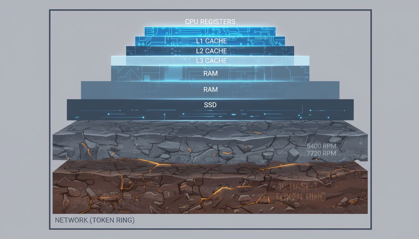
The 2009 Jeff Dean table reflected the hardware of that era. A lot has changed.
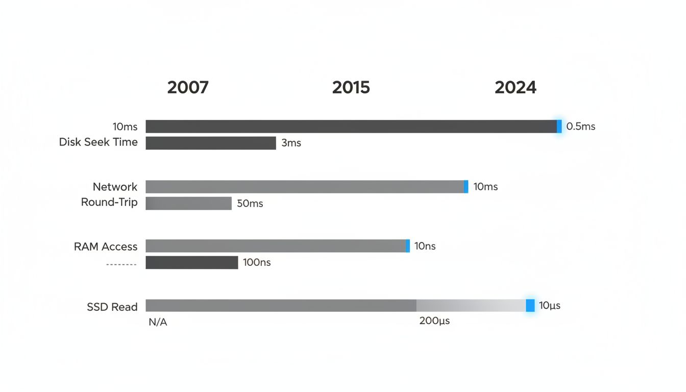
NVMe SSDs, which were not widely deployed in data centers in 2009, read sequentially at latencies an order of magnitude lower than the spinning disk numbers in the original table. Where the classic table listed disk seek time at around 10 milliseconds, a modern NVMe drive has seek latency under 100 microseconds. That is a 100x difference. The implication is that storage-backed caches, or even direct database reads with good access patterns, can be competitive with in-memory solutions in ways the classic table would suggest are impossible.
DRAM bandwidth has roughly tripled since 2009. Modern DDR5 memory has memory bandwidth over 50 GB/s per channel. L3 caches are dramatically larger, meaning the cache-hit versus cache-miss distinction plays out differently at scale. And critically, datacenter networking has transformed. In 2009, 1 Gbps was standard; 10 Gbps was high-end. Now 25 and 100 Gbps links are routine in cloud environments, and the actual round-trip time within a well-configured data center can be under 100 microseconds consistently.
None of this means memory is slow or disks are fast in absolute terms. It means the ratios have changed, and those ratios are what engineers actually use when making architectural decisions.
The Lesson Is Not What You Think
The easy takeaway is “measure everything,” which is true but not specific enough to be useful. The more precise lesson is about when rules of thumb expire and how quietly they do it.
The Jeff Dean numbers were never meant to be permanent. Dean himself updated the slide deck over the years, though the updates never propagated as virally as the original. The problem is that canonical teaching materials, Stack Overflow answers, and architecture blog posts continued citing the 2009 figures without timestamps. A number without a date is a number without a context, and hardware contexts change faster than documentation.
The fintech team’s mistake was not failing to measure. They were measuring throughout their development process. The mistake was that the priors they used to decide what to measure, and where to focus optimization effort, were built on a foundation that had shifted beneath them. They measured Redis latency extensively and confirmed it matched their predictions. What they didn’t question was whether those predictions were pointing them at the right problem.
Systems design requires reasoning under uncertainty, and rules of thumb are necessary tools. The answer is not to distrust all heuristics, it’s to know which shelf they came off of. A number you learned in a 2015 textbook that was citing a 2009 slide that was describing 2007 hardware is doing a lot of work for you. At some point it deserves a check-in.
Practically: if a performance assumption is load-bearing in an architecture decision, look up a current benchmark before committing. Brendan Gregg’s performance work, recent USENIX papers, and cloud provider documentation all contain measured numbers on contemporary hardware. The data exists; it just requires actually looking for it rather than reciting what you already know.
The engineers who built that fraud detection system were not bad engineers. They were doing what experienced engineers do: using accumulated knowledge efficiently. The trouble is that accumulated knowledge about hardware has a shelf life, and nobody stamps an expiration date on it when it enters your mental model.