Your Query Becomes a Number. A Lot of Numbers.
When you type a search query into a system backed by a vector database, the first thing that happens has nothing to do with databases. Your text gets handed to an embedding model, which converts it into a vector: an ordered list of floating-point numbers, typically somewhere between 384 and 1,536 dimensions depending on the model you’re using.
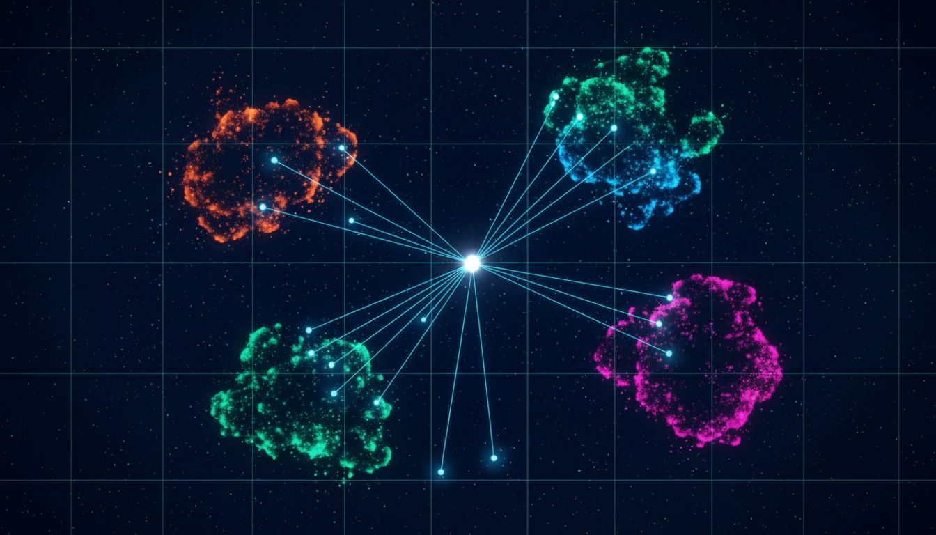
That vector is a coordinate in high-dimensional space. The position of that coordinate encodes meaning. Words or phrases with similar meaning end up close together in this space. “Dog” and “puppy” will be nearer to each other than “dog” and “carburetor.” The model learns these relationships during training by observing how words appear together across massive text corpora.
This is the foundation everything else rests on. If you understand that your query becomes a point in geometric space, the rest of how vector search works follows logically.
The Database Isn’t Storing Documents. It’s Storing Points.
Before any search happens, your data needs to go through the same transformation. Every chunk of text you want to make searchable, whether that’s a product description, a support ticket, a paragraph from a PDF, gets passed through the same embedding model and converted to a vector. Those vectors get stored in the database alongside a reference back to the original content.
This is why embedding model choice matters so much, and why you can’t mix models. A vector produced by OpenAI’s text-embedding-3-small lives in a completely different geometric space than one produced by Cohere’s embed-english-v3.0. Searching across them would be like trying to find the closest city on a globe using coordinates from a flat map.
When you run a semantic search, the database is finding which stored points are geometrically closest to your query point. The most common distance measure is cosine similarity, which compares the angle between two vectors rather than the raw distance. This is useful because it captures directional similarity regardless of magnitude. Two documents can be long or short, verbose or terse, and cosine similarity still captures whether they’re pointing in the same semantic direction.
The Brute-Force Approach and Why It Breaks Down
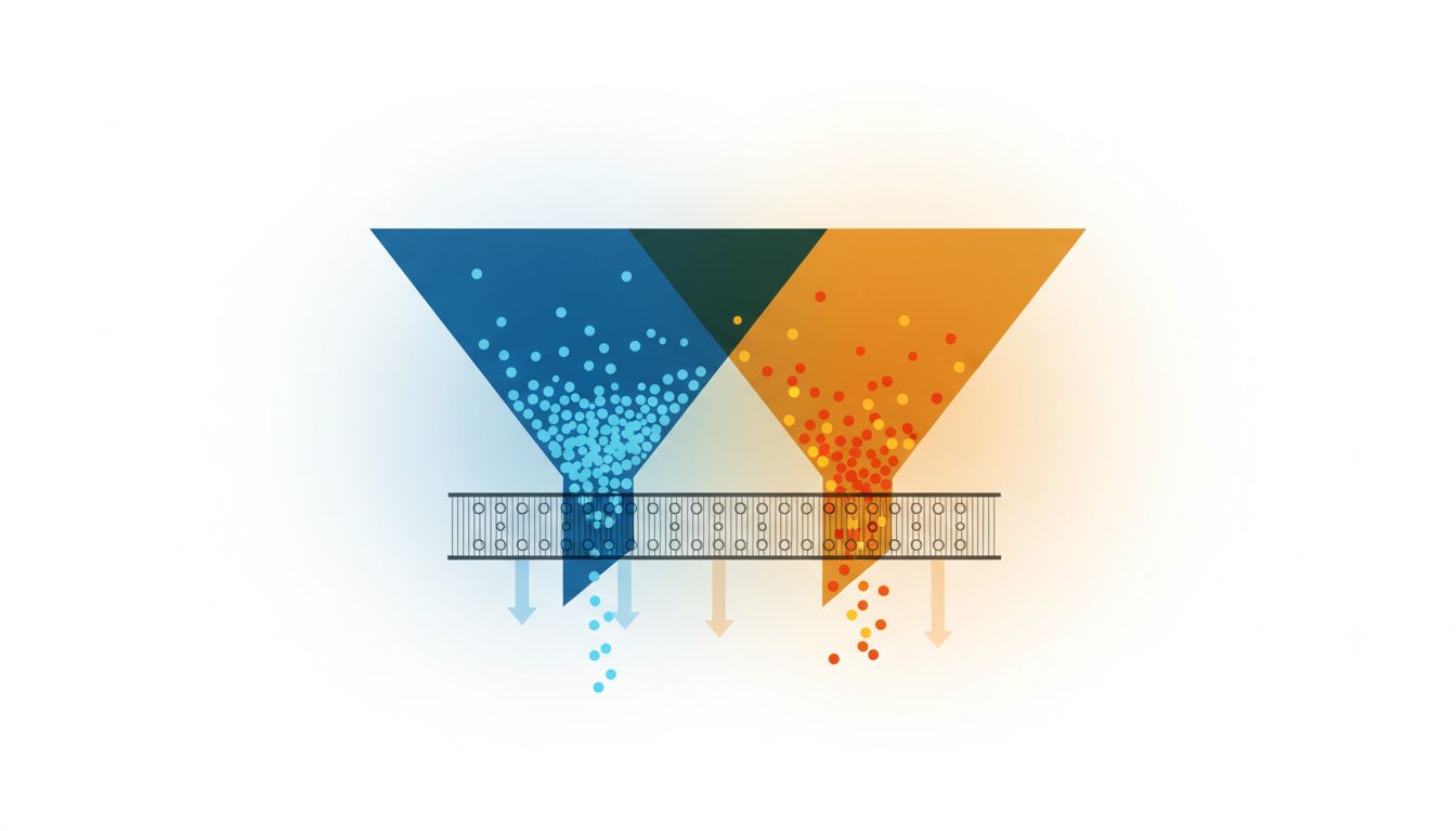
The naive way to find the nearest neighbors to your query vector is to compare it against every other vector in the database. Compute the distance to each one, sort, return the top results. This is called exact nearest-neighbor search, and for small datasets it works fine.
The problem is that it scales linearly. Double your stored vectors and you double your search time. For millions or billions of embeddings, that’s unusable. A 1,536-dimensional vector comparison isn’t free, and doing it a billion times per query would make real-time search impossible.
This is where approximate nearest-neighbor (ANN) algorithms come in, and this is where vector databases earn their complexity.
How HNSW Actually Navigates High-Dimensional Space
Most production vector databases use an algorithm called Hierarchical Navigable Small World, or HNSW. The name is dense but the idea is intuitive once you see it.
Imagine you’re trying to find a specific address in an unfamiliar city. You wouldn’t check every street. You’d zoom out to a map, find the right neighborhood, then the right block, then the right building. HNSW builds a graph structure that does something similar.
During indexing, HNSW creates multiple layers of a graph. The top layers are sparse, with connections only between vectors that are far apart in the dataset. Each lower layer is progressively denser. To search, you start at the top layer and greedily navigate toward your query vector, hopping between nodes along the connections that reduce distance fastest. As you find a better approximate neighborhood, you descend to a denser layer and refine your search.
The result is that instead of comparing against every vector, you follow a path through the graph that converges on the right region quickly. HNSW search complexity is roughly logarithmic, which makes a dramatic practical difference at scale.
You control a tradeoff with two parameters: ef_construction at index-build time (more connections means better accuracy but slower indexing and more memory) and ef_search at query time (searching a larger candidate set means more accurate results but slower queries). Tuning these is one of the first levers you pull when a vector search isn’t returning what you expect.
HNSW isn’t the only ANN approach. Pinecone has built proprietary indexing strategies. Weaviate supports HNSW natively. FAISS, Meta’s open-source library that underlies many implementations, supports several index types including IVF (Inverted File Index), which clusters vectors into buckets first and only searches the most relevant buckets. Each approach makes different tradeoffs between memory usage, query speed, and recall accuracy.
Recall, Not Accuracy, Is the Metric That Matters
Vector database performance is measured in recall, which is the fraction of the true nearest neighbors that an approximate search correctly returns. If exact search would return vectors A, B, and C as your top three, and your ANN search returns A, B, and D, your recall is 0.67.
In practice, 0.95 to 0.99 recall is achievable at reasonable speeds and memory costs. Whether you need 0.95 or 0.99 depends entirely on your application. A recommendation system might be fine with 0.95. A legal document search where missing a relevant precedent has real consequences probably needs to be closer to 1.0.
This is a genuine engineering decision, not a dial you just turn to maximum. Higher recall requires either slower queries, more memory, or both. Understanding this tradeoff lets you have an honest conversation about what your system actually needs rather than chasing precision for its own sake.
Filtering Makes Everything Harder
Here’s where many teams hit an unexpected wall. Vector search returns the semantically closest items, but you almost always need to combine semantic similarity with structured filters. Show me documents similar to this query, but only from the last 90 days, only in the user’s account, only with a status of “published.”
This is harder than it sounds, and it’s an active area of development across every major vector database.
The naive approach is post-filtering: run the ANN search to get candidates, then filter by metadata. The problem is that if most of your dataset gets filtered out, your top-k results after filtering might be terrible because you’re picking from a small unrepresentative pool. If you ask for the 10 most similar documents but 95% of your corpus gets filtered out, your ANN search needed to cast a much wider net.
Pre-filtering (applying filters before the vector search) has its own problem: it can break the graph structure that HNSW relies on. If you’re only searching a subset of nodes, the navigational connections built during indexing may not lead you to the right places efficiently.
Databases like Qdrant have built filtered HNSW that integrates metadata filters into the graph traversal. Pinecone uses a hybrid approach with metadata indexes. Weaviate supports filtering at query time with varying performance characteristics depending on filter selectivity. Which approach your database uses matters, and it’s worth reading the vendor’s documentation on filtered search specifically before committing to a solution.
What Hybrid Search Adds to the Picture
Pure semantic search has a real weakness: keyword precision. If a user searches for a specific product code, a person’s name, or a technical term that appears rarely in training data, vector similarity can let you down. The query might be embedded near related concepts, but not near the specific documents that contain the exact term.
Hybrid search solves this by combining vector search with traditional BM25 keyword search, then merging the two result sets. BM25 (the algorithm behind most full-text search, including Elasticsearch) rewards exact term matches weighted by frequency and document length. Combining it with vector similarity gives you semantic understanding plus keyword precision.
The merging step is called reciprocal rank fusion (RRF) in most implementations. Each document gets a score based on its rank in both result sets, and those scores get combined. The weighting between the two approaches is tunable. For queries that look like natural language questions, you want semantic search to dominate. For queries that look like specific identifiers or rare terms, you want keyword search to carry more weight.
If you’re building a search feature that users will actually type into, hybrid search is almost always worth the added complexity.
What This Means for Your Architecture
If you’re integrating a vector database into a product, here’s what you should carry forward:
Your embedding model and your database are coupled. Pick the model first based on your language needs and domain, then build around it. Switching models later means re-embedding your entire corpus.
Tune ef_search at query time, not just at index time. It’s the fastest lever for improving search quality in production without rebuilding your index.
Expect filtering to be your first scaling problem, not raw dataset size. Test filtered queries with realistic filter selectivity from the start, not just clean benchmark queries against the full corpus.
Recall is a product decision dressed up as a technical one. Decide what your use case actually requires and build your index parameters to hit that target, then stop.
Semantic search that feels effortless to users rests on a lot of concrete machinery. Understanding that machinery means you can debug it when it misbehaves, tune it when it’s slow, and make informed choices about which database and index strategy fits your actual workload.