
Softmax is one of those functions that gets introduced in ML tutorials as a one-liner: “it turns raw scores into probabilities that sum to 1.” That is technically true and practically incomplete. The function is doing several non-obvious things at once, and misunderstanding them leads to real bugs, overconfident models, and incorrect intuitions about how neural networks make decisions.
Here is what softmax is actually doing, in order of subtlety.
1. It Does Not Preserve Relative Differences, It Amplifies Them
Given a vector of raw scores (called logits) like [2.0, 1.0, 0.1], softmax does not just rescale these proportionally. It exponentiates each value first. So you are computing e^2.0, e^1.0, and e^0.1, which gives roughly [7.39, 2.72, 1.11], then dividing each by the sum to get probabilities around [0.66, 0.24, 0.10].
The score of 2.0 was twice the score of 1.0, but after softmax the corresponding probability is nearly three times as large. That non-linearity is the point: softmax is a winner-take-more function by design. In classification tasks this is useful because you want the model to commit. But it means that small changes in logits produce disproportionately large changes in the output distribution, especially when scores are spread far apart.
2. Only the Differences Between Logits Matter, Not the Values Themselves
This is the one that catches people off guard. If you add a constant to every logit, the softmax output is identical. Add 5 to [2.0, 1.0, 0.1] and you get [7.0, 6.0, 5.1]. The softmax of both vectors is the same, because exponentiation preserves ratios: e^(x+c) / sum(e^(y+c)) reduces to e^x / sum(e^y) after cancellation.
This has practical implications. You cannot interpret the absolute magnitude of logits as meaningful. A model that outputs [100, 99, 98] is expressing a much narrower preference than [3, 2, 1], even though in raw terms the first looks more decisive. What matters is the gap between scores. This is why temperature scaling in language models works the way it does: dividing logits by a temperature value T before applying softmax widens or narrows the gaps, which flattens or sharpens the resulting distribution. The relationship between temperature and model behavior is fundamentally a story about logit gaps, not logit magnitudes.
3. Softmax Probabilities Are Not Calibrated Confidence Scores
A softmax output of 0.97 for a given class does not mean the model is 97% likely to be correct. It means the model’s logits were shaped such that one class received a much higher score than the others. Whether that score actually corresponds to real-world accuracy is a separate question entirely, and in practice the answer is often no.
Models trained with cross-entropy loss and softmax tend to be overconfident, particularly on inputs far from the training distribution. A common fix is temperature scaling after training, which finds a single scalar that adjusts logit gaps to better align the model’s stated probabilities with its actual accuracy. This is a post-hoc calibration step. The model’s parameters do not change; only the interpretation of its outputs does. If you are building anything where the probability score matters for downstream decisions (medical diagnosis, fraud scoring, multi-step pipelines), you need to treat raw softmax outputs as uncalibrated and apply proper calibration. Confidence scores from AI systems are frequently decorative in practice, and softmax is a major reason why.
4. The Denominator Is a Global Operation, Which Causes Gradient Problems
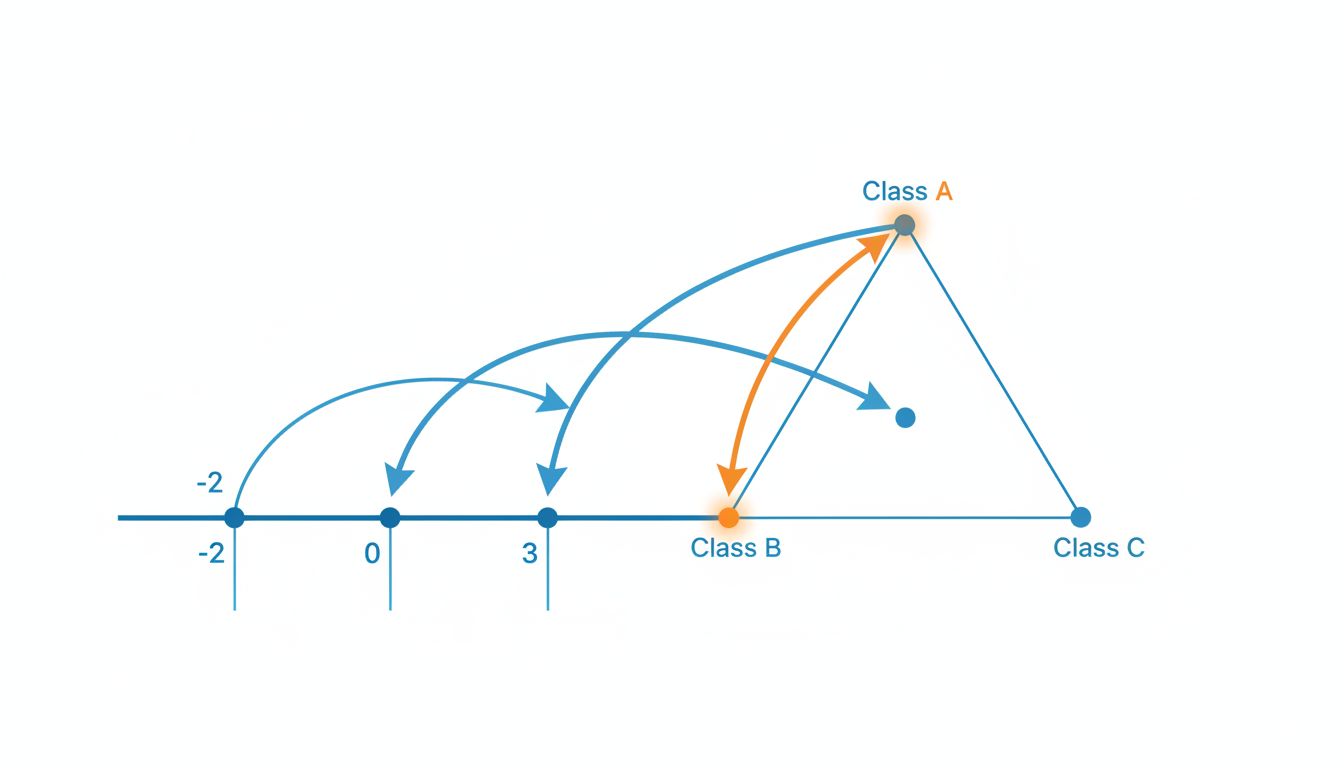
Softmax is computed across all classes simultaneously. The denominator, the sum of all exponentiated logits, couples every output unit to every other one. When you backpropagate through softmax during training, increasing the probability of one class necessarily decreases the probability of all others. That coupling is mathematically correct and semantically appropriate for single-label classification. For multi-label problems (where a photo can legitimately contain both a cat and a dog), applying softmax is a category error. Sigmoid applied independently per output is the right tool there.
The global normalization also makes softmax expensive when the number of classes is very large. Vocabulary-sized output layers in language models can have tens of thousands of classes. Computing the denominator over all of them at every training step is a significant cost. This is why approximate methods like sampled softmax, noise contrastive estimation, and hierarchical softmax exist. They are all strategies for approximating the denominator without summing over every class.
5. Softmax Treats Every Class as a Live Possibility
This is the subtlest behavioral issue. Even for classes that are completely irrelevant to a given input, softmax assigns them non-zero probability. In a 1000-class classifier, the 999 wrong classes collectively hold some probability mass. The model cannot express zero probability for anything. Numerically this is fine, but semantically it creates a situation where the model is always, to some degree, hedging across all options.
In practice this becomes a problem at inference time when you rely on the top softmax score as a rejection threshold. If a model is trained on cats and dogs and shown a photograph of a car, it will still assign probabilities summing to 1.0 across “cat” and “dog”. It cannot output “none of the above.” Systems that need to detect out-of-distribution inputs require additional machinery beyond raw softmax outputs, such as an explicit background class during training, energy-based scoring, or a separate out-of-distribution detector. This limitation is structural, not a matter of the model needing more data.
Softmax is elegant and usually the right default for single-label classification. But it is doing work that goes beyond normalization: it is amplifying score gaps, stripping absolute scale, and coupling every output to every other. Understanding those properties matters the moment you step outside the comfortable case of a well-trained, in-distribution classifier and start asking the model to do something more interesting.