

When you hit send on a prompt, you get back a blinking cursor, then words. The gap between those two things feels like waiting, the way you wait for a web page to load. But it’s not. What happens in those seconds is a specific computational process with identifiable stages, each with its own failure modes and tradeoffs. Understanding it makes you a better user of these systems, and if you’re building with them, it’s not optional knowledge.
Your Text Gets Turned Into Numbers First
Before any ‘intelligence’ happens, your prompt goes through tokenization. A tokenizer breaks your input into chunks called tokens, which map to integers in a vocabulary table. The word ‘cat’ might be one token. ‘Unbelievable’ might be three. Code and specialized vocabulary tend to fragment more than plain English.
This matters for a few reasons. GPT-4’s tokenizer (called tiktoken, and open-sourced by OpenAI) treats whitespace and punctuation as distinct tokens, which is why your tab-indented Python costs more to process than you might expect. And because the model only ever sees these integer IDs, not your original characters, it has no inherent understanding of spelling. It learned statistical relationships between token sequences, not letters. That’s why LLMs make character-level mistakes that feel bizarre given how ‘smart’ they seem otherwise. As you’re paying for tokens, not thinking, the tokenization step is where your billing starts.
The Prompt Gets Embedded Into a High-Dimensional Space
Once tokenized, each token ID gets converted into an embedding: a vector with hundreds or thousands of floating-point values. You can think of this as a coordinate in a very high-dimensional space where semantic relationships are encoded as distances. Tokens with similar meanings tend to cluster; tokens used in similar contexts end up nearby.
For GPT-4-class models, these embedding vectors are in the thousands of dimensions. The full prompt, now a sequence of these vectors, is what actually enters the neural network. This is also where positional encoding gets added: information about where in the sequence each token sits, since transformers (the underlying architecture) don’t have an intrinsic sense of order the way a recurrent network would.
The embedding layer is pre-trained and frozen during inference. It’s not being updated when you use the model. What you’re doing is performing a lookup and arithmetic operations, not anything that changes the model.
Attention Is the Actual Work, and It’s Expensive
The transformer architecture’s key mechanism is self-attention, and this is where most of the computation happens. For every token in your prompt, the model computes how much that token should ‘attend to’ every other token when building its representation of meaning.
Concretely: if your prompt contains the sentence ‘The bank by the river was slippery,’ the token ‘bank’ needs to figure out it’s referring to a riverbank, not a financial institution. It does this by computing attention scores against every other token in the context. ‘River’ should get a high score; ‘financial’ (if it appeared) would get a low one. These scores are used to weight a weighted sum of value vectors, producing an updated representation that carries contextual meaning.
Now scale that up. A model with 96 attention layers and multi-head attention (GPT-4 uses something in this range, though exact architecture details aren’t public) runs this computation repeatedly, stacking layers of contextual refinement. The computational cost grows quadratically with sequence length, which is why processing a 100,000-token context window takes meaningfully more time and GPU memory than processing a 1,000-token one. For a deeper look at what that actually means, what an LLM actually does with 100,000 tokens covers the memory mechanics specifically.
The Forward Pass: One Big Matrix Multiply
Self-attention is followed by feed-forward layers, and together these form a single transformer block. Modern models stack dozens to hundreds of these blocks. Running the full network on your prompt is called the forward pass, and at its core it’s a very large sequence of matrix multiplications.
This is why GPUs matter so much. Matrix multiplication parallelizes beautifully across the thousands of CUDA cores on a modern GPU. An A100, which is the workhorse of most large-scale inference infrastructure, can do around 312 teraflops of bfloat16 computation. Even so, a single forward pass through a large model on a long prompt can take a perceptible fraction of a second, just for the computation before any output starts.
The output of the final transformer block, for the last token in your sequence, is a vector that gets projected into the vocabulary space. A matrix multiplication maps that vector to a score for every possible next token (the vocabulary might be 100,000 entries or more). A softmax operation converts those scores into probabilities.
Sampling: Where Randomness Lives
You might expect the model to just pick the highest-probability next token. Sometimes it does, if temperature is set to zero. More often, sampling is involved.
Temperature is a scalar that modifies the probability distribution before sampling. High temperature (above 1.0) flattens the distribution, making lower-probability tokens more competitive. Low temperature sharpens it, making the model more deterministic. At temperature 0 you get pure greedy decoding; at temperature 1.0 you’re sampling from the raw distribution.
Top-p sampling (also called nucleus sampling) is another common technique: instead of sampling from all 100,000+ tokens, you only sample from the smallest set of tokens whose cumulative probability exceeds a threshold, say 0.9. This prevents the model from occasionally sampling bizarre low-probability tokens while maintaining diversity.
These parameters are what ‘creativity’ and ‘determinism’ sliders in various interfaces are actually controlling. When you complain that a model gave you a different answer to the same question, that’s usually sampling at work, not inconsistency in any deep sense.
Autoregressive Generation: One Token at a Time
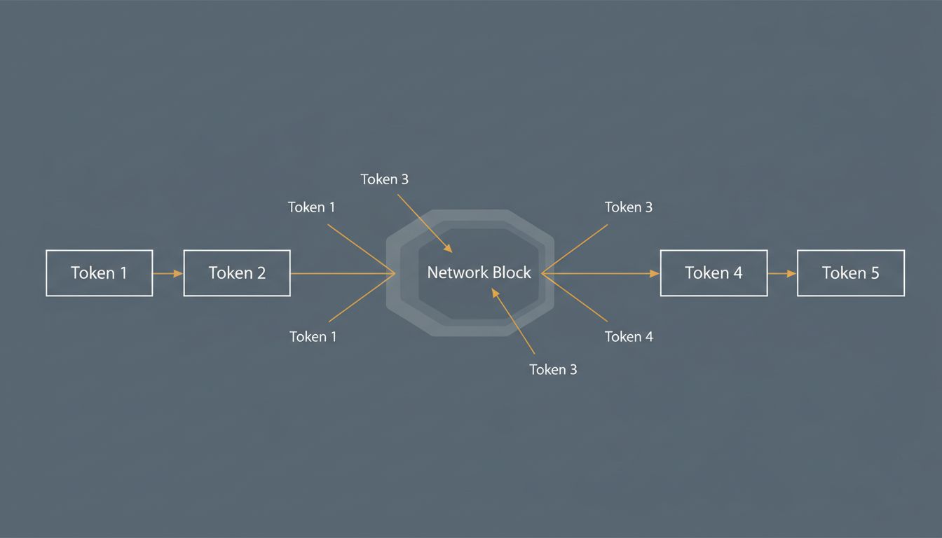
Here’s the part most people find surprising when they first encounter it: the model generates your entire response one token at a time, running the full forward pass for each token. To generate the second token, it runs the network again on the original prompt plus the first token it already generated. For the third token, the original prompt plus the first two tokens. And so on.
This is called autoregressive generation, and it’s why streaming responses (where text appears word by word in real time) reflect the actual computation, not just a UX trick. The model genuinely finishes computing each token before it knows what the next one will be. There’s no separate ‘compose the whole response’ step.
KV-caching (key-value caching) exists to make this less catastrophically slow. During the forward pass for token N, intermediate computations for tokens 1 through N-1 are cached and reused when computing token N+1. Without this, generation would scale badly with response length. With it, each new token requires significantly less computation than starting from scratch.
This architecture has an interesting implication: the model doesn’t plan its response before it starts writing it. It’s committing to each word sequentially, which is why you can sometimes watch a model start a sentence and then write itself into a corner. It’s not choosing poorly from a set of fully-formed options; it’s making locally plausible choices that can compound into globally awkward outputs.
What This Means for How You Use These Systems
If you’ve made it here, a few things should now make more intuitive sense.
Why prompt length affects cost and latency in a nonlinear way: attention is quadratic in sequence length. A prompt twice as long can take more than twice as long to process.
Why models are bad at counting characters or noticing specific patterns: they operate on tokens, not characters. Ask a model how many times the letter ‘e’ appears in a word and it’s doing something more like reconstruction from statistics than scanning.
Why the same prompt with temperature 0 gives you the same answer every time, but with temperature 1.0 gives you different answers: that’s sampling, not inconsistency.
Why streaming feels natural even though you’re technically waiting for computation: you’re seeing actual token-by-token generation, not a buffer being released.
And perhaps most importantly: the model isn’t thinking, then writing. It’s writing as it thinks, one token at a time, in a single left-to-right pass. There’s no scratchpad it’s hiding from you, no moment where it drafted three options and chose the best one (unless you’re using something like chain-of-thought prompting, which explicitly forces intermediate tokens). What you see in the stream is the computation itself.
That’s not a limitation to dismiss. It’s a design to understand.