
The Geometry of Meaning
When you store text in a vector database, you’re not storing words. You’re storing a list of numbers, typically hundreds or thousands of them, that represent where that text lands in a high-dimensional geometric space. Two pieces of text are considered “similar” if their vectors are close together in that space.
This sounds reasonable until you ask: close according to what?
Most vector databases default to one of three distance metrics: cosine similarity, Euclidean distance, or dot product. Each one measures something slightly different. Each one will return different results for the same query. And most systems ship with a default that their engineers chose without knowing what your data looks like or what “similar” means for your specific use case.
This is not a minor implementation detail. The choice of distance metric is a modeling decision, and getting it wrong quietly degrades your retrieval quality in ways that are genuinely hard to debug.
What These Metrics Actually Measure
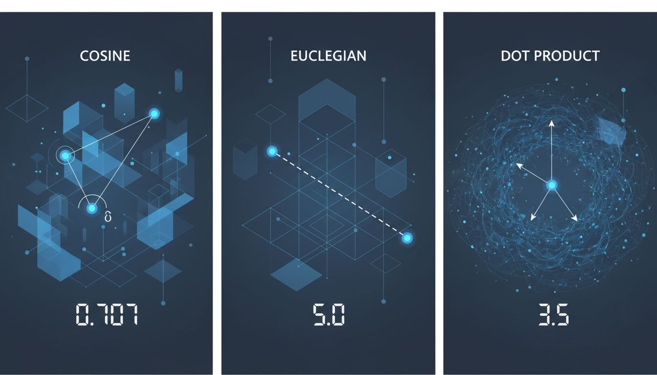
Cosine similarity measures the angle between two vectors, ignoring their magnitude. Two documents that use the same vocabulary in similar proportions will score high cosine similarity even if one is a tweet and one is a dissertation. The length of the document doesn’t matter, only the direction the vector points.
Euclidean distance measures the straight-line distance between two points in space. Magnitude matters here. A short document and a long document covering the same topic might end up far apart in Euclidean space because the embedding for the longer one has larger component values, even if they’re directionally aligned.
Dot product combines both angle and magnitude. It rewards vectors that point in the same direction and have large values. In practice, this means it tends to favor longer, denser documents over short ones, regardless of relevance.
None of these is correct in the abstract. They’re tools, and using the wrong one for your data is like measuring your living room with a thermometer: you’ll get a number, but not a useful one.

The Embedding Model Is Half the Problem
Here’s the part that trips up a lot of practitioners: the distance metric you should use depends heavily on how your embedding model was trained.
Some models are trained to produce unit-normalized vectors, meaning every embedding has a magnitude of exactly 1. For these models, cosine similarity and dot product produce identical rankings. The choice between them is meaningless. Other models produce embeddings where magnitude carries information, and those should not be compared with cosine similarity unless you normalize first.
OpenAI’s text-embedding-ada-002, for a concrete example, produces normalized vectors. Cosine similarity and dot product are equivalent for it. But if you’re using a model that wasn’t trained with normalization in mind and you apply cosine similarity, you’re throwing away information the model actually encoded.
This is compounded by the fact that embedding models are trained on specific objectives. A model trained for semantic textual similarity (determining whether two sentences mean the same thing) behaves very differently from one trained for information retrieval (finding documents relevant to a query). The first is symmetric: similarity of A to B equals similarity of B to A. The second is often asymmetric: a short query might not be “close” to a long relevant document in embedding space because their representations were constructed differently.
Models in the BEIR benchmark family, designed for retrieval tasks, often benefit from asymmetric setups where queries and documents are embedded with different encoders. Feeding both through the same encoder and then computing cosine similarity is a category error, not just a performance hit.
As explained in Embeddings Don’t Measure Meaning, They Measure Habit, these vectors encode statistical patterns from training data. “Similar” in embedding space means “appeared in similar contexts in the training corpus,” which is related to but not identical to the semantic similarity you probably want.
When Nearest Neighbor Isn’t the Right Concept
Vector search is built on the nearest neighbor problem: given a query vector, find the stored vectors that are closest to it. This is elegant and computationally tractable (with approximation algorithms like HNSW or IVF). But nearest neighbor assumes that proximity in the embedding space correlates with what you care about, and that assumption breaks in interesting ways.
Consider a document retrieval system for a legal firm. A query about “contract termination” might sit geometrically close to documents about “employment termination,” “product warranties,” and “subscription cancellations,” because these topics share vocabulary and surface-level semantics. The model has no concept of which of these the user actually wanted. It found neighbors. Whether those neighbors are relevant is a different question entirely.
The problem is worse in high-dimensional spaces due to a phenomenon called the curse of dimensionality. As dimensions increase, the ratio between the nearest neighbor distance and the farthest neighbor distance approaches 1. In very high dimensions, almost all points are roughly equally far from your query point. Your “nearest” neighbors aren’t meaningfully closer than the rest of the database. Many practical embedding dimensions (768, 1536) are high enough for this to matter.
This is why filtering matters. Doing pure vector search across your entire corpus often performs worse than filtering to a relevant subset first and then running vector search within that subset. The geometry works better when you’ve narrowed the playing field.
Approximate Search Adds Another Layer
Most production vector databases don’t do exact nearest neighbor search. They do approximate nearest neighbor search (ANN). Finding the mathematically exact nearest neighbor in a billion-vector database is slow enough to be impractical, so systems like Pinecone, Weaviate, Qdrant, and Milvus use indexing structures that trade accuracy for speed.
HNSW (Hierarchical Navigable Small World graphs) is the dominant approach. It builds a multi-layer graph where each layer is a subset of the data, and search navigates down from coarse layers to fine ones. It’s fast and works well in practice. But it has parameters, most importantly ef_construction and M, that control the quality of the index versus the speed of building it. The defaults are reasonable but not universally optimal.
More importantly: ANN search can miss the true nearest neighbor. That’s the whole tradeoff. In most retrieval contexts this is acceptable because the tenth-closest result is usually as good as the ninth. But in some applications, like finding exact duplicate content or searching for specific code snippets, you actually need exact search, and running ANN there will silently fail without telling you it missed anything.
Practitioners routinely discover that their recall degrades over time as they add more data to an index without rebalancing. The index was tuned for a certain data distribution and density, and as that changes, the approximation quality drifts. This is a distributed systems reliability problem in disguise: things work fine at small scale and fail subtly at large scale.
Metadata Filtering Breaks the Geometry
Most real applications combine vector search with metadata filters. You don’t just want the ten most similar documents globally, you want the ten most similar documents written after 2022, or tagged with a specific category, or belonging to a specific user’s namespace.
The naive implementation runs the metadata filter after retrieving the top-k vector results. If your filter is selective (say, only 5% of your corpus matches), this fails badly. You might retrieve the 100 nearest vectors globally and find that only two of them pass the filter, even though there are fifty highly relevant documents in that 5% subset that weren’t in your top 100.
The correct approach is pre-filtering: restrict the search space to matching documents first, then run vector search within that subset. But pre-filtering with HNSW is non-trivial because the graph structure doesn’t respect arbitrary metadata partitions. Some databases handle this better than others. Qdrant, for instance, has built-in support for filtered search that avoids this degradation. Others silently give you bad results.
This is the kind of thing you won’t notice in development when your dataset is small and your filters are loose, and will notice in production when a high-value query returns irrelevant results and someone asks why.
What This Means in Practice
The core issue is that “semantic search” has become a black box that practitioners wire up without examining the assumptions inside it. Here’s what actually needs to match for the system to work correctly:
Your embedding model needs to be trained for your retrieval task, not just any text task. Semantic similarity models and retrieval models are different products.
Your distance metric needs to match how your embedding model was trained. Check whether your model produces normalized vectors. If it does, cosine and dot product are equivalent. If it doesn’t, this choice matters.
Your ANN index parameters need to be tuned for your data size and distribution, and revisited when either changes significantly.
Your metadata filtering strategy needs to be pre-filtering, not post-filtering, if your filters are selective.
And fundamentally, you need an evaluation set: a collection of queries with known-good results, so you can actually measure whether your retrieval is working rather than assuming it is. Without this, you’re flying blind. Any of the above problems will manifest as “the search feels off” feedback from users, which is nearly impossible to diagnose without ground truth.
Vector databases are genuinely useful infrastructure. But they’re tools that implement specific mathematical operations, not magic boxes that understand what your users mean. The gap between the geometry and the meaning is your responsibility to bridge.